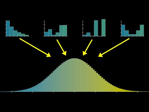
But what is the Central Limit Theorem?
What this covers
A visual introduction to probability's most important theorem Help fund future projects: https://www.patreon.com/3blue1brown Special thanks to these lovely supporters: https://www.3blue1brown.com/lessons/clt#thanks An equally valuable form of support is to simply share the videos.
Galton board shown in the video: https://amzn.to/3ZJK8nY
Thanks to these viewers for their contributions to translations Hebrew: David Bar-On, Omer Tuchfeld Hindi: Tapender1 Italian: anna-lombardo
-----------------
Timestamps 0:00 - Introduction 1:53 - A simplified Galton Board 4:14 - The general idea 6:15 - Dice simulations 8:55 - The true distributions for sums 11:41 - Mean, variance, and standard deviation 15:54 - Unpacking the Gaussian formula 20:47 - The more elegant formulation 25:01 - A concrete example 27:10 - Sample means 28:10 - Underlying assumptions
Correction: 6:37 The narration should say "skewed left" Correction: 7:15 Again, the narration should say "skews a tiny bit left"
------------------
These animations are largely made using a custom python library, manim. See the FAQ comments here: https://www.3blue1brown.com/faq#manim https://github.com/3b1b/manim https://github.com/ManimCommunity/manim/
You can find code for specific videos and projects here: https://github.com/3b1b/videos/
Music by Vincent Rubinetti. https://www.vincentrubinetti.com/
Download the music on Bandcamp: https://vincerubinetti.bandcamp.com/album/the-music-of-3blue1brown
Stream the music on Spotify: https://open.spotify.com/album/1dVyjwS8FBqXhRunaG5W5u
------------------
3blue1brown is a channel about animating math, in all senses of the word animate. And you know the drill with YouTube, if you want to stay posted on new videos, subscribe: http://3b1b.co/subscribe
Various social media stuffs: Website: https://www.3blue1brown.com Twitter: https://twitter.com/3blue1brown Reddit: https://www.reddit.com/r/3blue1brown Instagram: https://www.instagram.com/3blue1brown Patreon: https://patreon.com/3blue1brown Facebook: https://www.facebook.com/3blue1brown
Source description (no synthesized summary yet).
The Central Limit Theorem states that when summing many independent random variables from any distribution, the resulting distribution converges to a normal (bell curve) distribution, regardless of the original distribution's shape, characterized by a specific mathematical formula involving e and π.
- Increasing the number of summed variables causes any initial distribution to approximate a bell curve shape
- The mean and standard deviation of the sum follow predictable formulas: mean scales linearly with n, standard deviation scales with √n
- The theorem holds for arbitrary starting distributions, whether uniform or heavily skewed
This asset isn't compiled yet
You're seeing its claims, ranked. Compile it to build the argument threads, weight them, and check each claim against your library — the full view.
A Galton board demonstrates that even when individual outcomes are chaotic and random with unknowable results, precise statements can be made about the distribution of large numbers of events across different outcome categories.
“This is a Galton board. Maybe you've seen one before, it's a popular demonstration of how, even when a single event is chaotic and random, with an effectively unknowable outcome, it's still possible to make precise statements about a large number of events, namely how the relative proportions for many different outcomes are distributed.”
The central limit theorem does not require that the initial distribution be uniform or fair—it holds for weighted distributions with non-trivial probability structures.
“Usually if you think of rolling a die you think of the six outcomes as being equally probable, but the theorem actually doesn't care about that. We could start with a weighted die, something with a non-trivial distribution across the outcomes, and the core idea still holds.”
The Central Limit Theorem is the core principle explaining why the normal distribution is so common: almost nothing you can do to the initial distribution changes the shape that the sum of many variables tends towards.
“This, this right here is what the central limit theorem is all about. Almost nothing you can do to this initial distribution changes the shape we tend towards.”
For a probability distribution, the area under the curve must equal 1, representing the total probability, and for the function e^(-x²), the area is √π, not 1.
“Before we can interpret this as a probability distribution, we need the area under the curve to be 1... As it stands with the basic bell curve shape of e to the negative x squared, the area is not 1, it's actually the square root of pi. I know, right? What is pi doing here? What does this have to do with circles?”
Assumption 3 of the central limit theorem: the variance of the random variables being summed must be finite, meaning the sum in the variance formula does not diverge to infinity.
“The third assumption is actually fairly subtle. It's that the variance we've been computing for these variables is finite. This was never an issue for the dice example because there were only six possible outcomes. But in certain situations where you have an infinite set of outcomes, when you go to compute the variance, the sum ends up diverging off to infinity.”
Some probability distributions have infinite sets of outcomes and infinite variance, and in these cases, even if independence and identical distribution hold, the sum may not converge to a normal distribution.
“These can be perfectly valid probability distributions, and they do come up in practice. But in those situations, as you consider adding many different instantiations of that variable and letting that sum approach infinity, even if the first two assumptions hold, it is very much a possibility that the thing you tend towards is not actually a normal distribution.”
As sample size increases in computing an empirical average, the standard deviation of the average decreases, allowing more precise estimates of the true expected value.
“In particular, it's worth your time to take a moment mulling over what the standard deviation for this empirical average is, and what happens to it as you look at a bigger and bigger sample of die rolls.”
When summing only a small number of random variables (e.g., 2-3), the distribution of the sum strongly depends on the initial distribution and does not yet look like a bell curve.
“Let me start by rolling things back so that the distribution on the bottom represents a relatively small sum, like adding together only three such random variables. Notice what happens as I change the distribution we start with. As it changes, the distribution on the bottom completely changes its shape. It's very dependent on what we started with.”
For a sum of n independent random variables from the same distribution with mean μ and standard deviation σ, the resulting sum has mean = n·μ and standard deviation = √n·σ.
“Putting some actual formulas to it, if we know the mean of our underlying random variable, we call it mu, and we also know its standard deviation, and we call it sigma, then the mean for the sum on the bottom will be mu times the size of the sum, and the standard deviation will be sigma times the square root of that size.”
The first assumption of the Central Limit Theorem is that all random variables being summed are independent—the outcome of one process does not influence the outcome of any other process.
“The first one is that all of these variables that we're adding up are independent from each other. The outcome of one process doesn't influence the outcome of any other process.”
For a continuous probability distribution, the area under the curve between two values equals the probability that a value falls between those two values, so the total area under the curve must equal 1.
“Unlike discrete distributions, when it comes to something continuous, you don't ask about the probability of a particular point. Instead, you ask for the probability that a value falls between two different values. And what the curve is telling you is that that probability equals the area under the curve between those two values... The main point right now is that the area under the entire curve represents the probability that something happens, that some number comes up. That should be 1, which is why we want the area under this to be 1.”
The normal distribution (bell curve) is one of the most prominent distributions in probability and appears in many seemingly unrelated contexts, such as human heights in similar demographics and the distribution of distinct prime factors in large numbers.
“the normal distribution is, as the name suggests, very common, it shows up in a lot of seemingly unrelated contexts. If you were to take a large number of people who sit in a similar demographic and plot their heights, those heights tend to follow a normal distribution. If you look at a large swath of very big natural numbers, and you ask how many distinct prime factors does each one of those numbers have, the answers will very closely track with a certain normal distribution.”
The standard normal distribution is the special case where σ = 1, and all possible normal distributions are parameterized by two parameters: μ (mean) and σ (standard deviation).
“The special case where sigma equals 1 has a specific name, we call it the standard normal distribution, which plays an especially important role for you and me in this lesson. And all possible normal distributions are not only parameterized with this value sigma, but we also subtract off another constant mu from the variable x, and this essentially just lets you slide the graph left and right so that you can prescribe the mean of this distribution. So in short, we have two parameters, one describing the mean, one describing the standard deviation, and they're all tied together in this big formula involving an e and a pi.”
When interpreting bar charts of distributions, the area of each bar (not its height) represents the probability of that outcome, and the y-axis represents probability density rather than probability.
“Also, by the way, in anticipation for the animation I'm trying to build to here, the way I'm representing things on that lower plot is that the area of each one of these bars is telling us the probability of the corresponding value rather than the height. You might think of the y-axis as representing not probability but a kind of probability density.”
For a fair die rolled 100 times, the sum of results has mean = 350 (100 × 3.5) and standard deviation ≈ 17.1 (10 × 1.71), allowing prediction that with 95% confidence the sum falls between approximately 316 and 384.
“Its mean will be 100 times mu, which is 350, and its standard deviation will be the square root of 100 times sigma, so 10 times sigma, 17.1. Remembering our handy rule of thumb, we're looking for values two standard deviations away from the mean, and when you subtract 2 sigma from mean, you end up with about 316, and when you add 2 sigma you end up with 384.”
The 68-95-99.7 rule states that for a normal distribution, approximately 68% of values fall within 1 standard deviation of the mean, 95% within 2 standard deviations, and 99.7% within 3 standard deviations.
“For questions like this, there's a handy rule of thumb about normal distributions, which is that about 68% of your values are going to fall within one standard deviation of the mean, 95% of your values, the thing we care about, fall within two standard deviations of the mean, and a whopping 99.7% of your values will fall within three standard deviations of the mean.”
The base e in the formula e^(-x²/2σ²) is not inherently special; the same family of bell curves can be produced using any other positive constant as the base, but e is chosen because it makes the constant σ have a readable meaning—σ becomes the standard deviation of the distribution.
“And in that sense, the number e is not really all that special for our formula. We could replace it with any other positive constant, and you'll get the same family of curves as we tweak that constant. Make it a 2, same family of curves. Make it a 3, same family of curves. The reason we use e is that it gives that constant a very readable meaning. Or rather, if we reconfigure things a little bit so that the exponent looks like negative 1 half times x divided by a certain constant, which we'll suggestively call sigma squared, then once we turn this into a probability distribution, that constant sigma will be the standard deviation of that distribution.”
Many people incorrectly assume variables are normally distributed without proper justification, which the speaker cautions against.
“But I do want to caution you against the fact that many times people seem to assume that a variable is normally distributed, even when there's no actual justification to do so.”
The Galton board, despite being used as a pedagogical illustration, actually violates the independence and identical distribution assumptions because a ball's trajectory and peg interactions are highly dependent and non-uniform across pegs.
“One situation where these assumptions are decidedly not true would be the Galton board. I mean, think about it. Is it the case that the way a ball bounces off of one of the pegs is independent from how it's going to bounce off the next peg? Absolutely not. Depending on the last bounce, it's coming in with a completely different trajectory. And is it the case that the distribution of possible outcomes off of each peg are the same for each peg that it hits? Again, almost certainly not.”
A random variable is shorthand for a random process where each outcome is associated with a number.
“The setup is that we have a random variable, and that's basically shorthand for a random process where each outcome of that process is associated with some number.”
The function e^x describes exponential growth, and when the exponent is made negative (e^-x), it describes exponential decay in both directions.
“The function e to the x, or anything to the x, describes exponential growth, and if you make that exponent negative, which flips around the graph horizontally, you might think of it as describing exponential decay.”
The mean of a fair six-sided die is 3.5, calculated as the weighted sum of outcomes: (1/6)×1 + (1/6)×2 + ... + (1/6)×6 = 3.5.
“Step 1 with a problem like this is to find the mean of your initial distribution, which in this case will look like 1 6th times 1 plus 1 6th times 2 on and on and on, and works out to be 3.5.”
The standard deviation is the square root of variance and can be interpreted as a distance on a diagram (unlike variance which has squared units); it is denoted by the Greek letter sigma.
“So another way to measure spread is what's called the standard deviation, which is the square root of this value. That can be interpreted much more reasonably as a distance on our diagram, and it's commonly denoted with the Greek letter sigma, so you know m for mean as for standard deviation, but both in Greek.”
By the end of the lesson, viewers should be able to determine a range of values where the sum of 100 dice rolls falls with 95% confidence, whether using a fair die or weighted die.
“For example, here's the kind of question I want you to be able to answer by the end of this video. Suppose you rolled a die 100 times and you added together the results. Could you find a range of values such that you're 95% sure that the sum will fall within that range?... The neat thing is you'll be able to answer this question whether it's a fair die or if it's a weighted die.”
In a simplified Galton board model where each ball has a 50-50 probability of bouncing left or right at each peg, the final position equals the sum of all the individual random choices (each contributing ±1).
“In this model we will assume that each ball falls directly onto a certain central peg, and that it has a 50-50 probability of bouncing to the left or to the right, and we'll think of each of those outcomes as either adding one or subtracting one from its position... we can think of its final position as basically being the sum of all of those different numbers”
The variance of a distribution measures spread by computing the expected value of the squared difference between each outcome and the mean; squaring makes the math nicer than using absolute values.
“One of them is called the variance. The idea there is to look at the difference between each possible value and the mean, square that difference, and ask for its expected value. The idea is that whether your value is below or above the mean, when you square that difference, you get a positive number, and the larger the difference, the bigger that number. Squaring it like this turns out to make the math much much nicer than if we did something like an absolute value”
When interpreting distributions graphically, higher values in the initial distribution become more probable in the sum distribution, because the weighted sum in the convolution operation emphasizes those values.
“If higher values are more probable, that weighted sum is going to be bigger. If lower values are more probable, that weighted sum is going to be smaller.”
For non-uniform distributions, the probability of different sums is calculated by going through all possible pairs of outcomes that sum to the same value and multiplying the individual probabilities for each outcome, then adding these products together—a computation called a convolution.
“You do essentially the same thing, you go through all the distinct pairs of dice which add up to the same value. It's just that instead of counting those pairs, for each pair you multiply the two probabilities of each particular face coming up, and then you add all those together. The computation that does this for all possible sums has a fancy name, it's called a convolution”
Heights of people in similar demographic groups follow a normal distribution when plotted across a large population.
“If you were to take a large number of people who sit in a similar demographic and plot their heights, those heights tend to follow a normal distribution.”
The number of distinct prime factors in large natural numbers closely tracks a normal distribution.
“If you look at a large swath of very big natural numbers, and you ask how many distinct prime factors does each one of those numbers have, the answers will very closely track with a certain normal distribution.”
After completing this lesson on the Central Limit Theorem fundamentals, the speaker plans a follow-up video explaining why the normal distribution formula has the specific form it does, why π appears in it, and how this connects to a previous promised video on convolutions.
“Next up, I'd like to explain why it is that this particular function is the thing that we tend towards, and why it has a pi in it, what it has to do with circles.”
Simulations become imprecise as sample size grows (at 3000 samples, the distribution looks bell-curved but buckets appear spiky), raising questions about whether spikiness reflects true distribution or simulation artifact.
“Illustrating things with a simulation like this is very fun, and it's kind of neat to see order emerge from chaos, but it also feels a little imprecise. Like in this case, when I cut off the simulation at 3000 samples, even though it kind of looks like a bell curve, the different buckets seem pretty spiky, and you might wonder, is it supposed to look that way, or is that just an artifact of the randomness in the simulation?”
The goal of the Galton board model is not to accurately model physics but to provide a simple example to illustrate the Central Limit Theorem.
“And for those of you who are inclined to complain that this is a highly unrealistic model for the true Galton board, let me emphasize the goal right now is not to accurately model physics, the goal is to give a simple example to illustrate the central limit theorem, and for that, idealized though this might be, it actually gives us a really good example.”